
For this analysis, I will be applying a Monte Carlo method to Bitcoin’s daily increment dollar rate. The main goal here is trying to calculate its most likely price for the late year 2018. You can find the code I used on GitHub.
What is a daily increment
In our case, the increment will show how the price was changed, proceeding from one observation to another. Since we will be inspecting daily increments, increment itself will be calculated daily. For this we will use the most basic formula:
![]()
Ideally, the daily increment price of financial assets should fit into the regular distribution, but the reality is far from it. Actual daily increments will have more “heavy” tails, meaning that more extreme events will have a higher probability than the ones predicted by standard distribution rule. As you can see in the image below, distributions will not be similar to each other.

What is the Monte Carlo method
According to Wikipedia, Monte Carlo method is a broad class of computational algorithms that rely on repeated random sampling to obtain numerical results. Its essential idea is using randomness to solve problems that might be deterministic in principle.
In Monte Carlo finance field simulation, we assume that both past and future behavior of the asset’s price will remain the same. Thus we will generate a number scenarios of the future, that is similar to the past. In Maths, those type of variations is called random walks.
Simulation begins
In order to simulate each of our random walks, we (separate thanks to fintech guys from Elinext) will be taking random increments, from a huge pool of price increases from the year 2010 until today, add one increment for each day in the future and multiply them cumulatively, to obtain increment price options until the very end of the year 2018. This data will be multiplied by the current bitcoin price, to receive simulated future prices. And then we will repeat this process 100000 times. In the end, we will get 100000 price prediction variants, obtained with the help of these random walks.
Random Walks
First 200 walks look like this:

This chart did not give us a lot of information, since exponential growth in some of the random walks made the scale of the chart too big, while most of the random walks ended way below the highest point. The logarithmic scale of the vertical axes will give us a better understanding of the situation:

Predicted prices final distribution
From what we can see, the final price for most of the random walks was between 10k and 100k USD. Now we build a histogram, showing the distribution of final price predictions in all of our 100000 random walks we created earlier.

The problem remains the same, therefore we cannot make any conclusions. We rebuild the chart using a logarithmic scale for the horizontal axes. This way it should look more coherent:
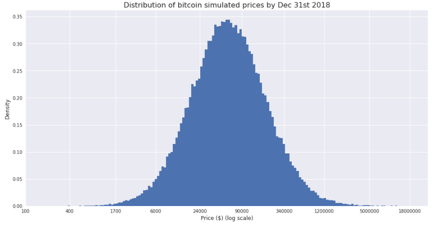
It looks like the price will vary from 24k to 90k USD. There is a couple of things we can do to find out an even more accurate result. One of the options is to simply calculate the median – 58,843 USD. Another option is to find the probability density function and price calculation, corresponding to the maximum of this function. You can see the result of all this below:

Estimates for the most probable price are identical and both are above $ 50,000.
It is important to note that this estimate should not be taken separately, but rather used as a way of finding confidence intervals in which with a certain probability chance you will find the future price. In this case, the 80% confidence interval for the bitcoin price will have borders from 13,200 to 271,277 USD. Another way to look at this is the probability that the price at the end of the year will be below 13200, is equal to the probability that the price will be higher than 271277 USD (if the price will move in the future in the same way as in the past).
Knowing the probability density function, we can now, for example, calculate the probability that the price will be below a certain level by the end of the year.
In particular, if we want to calculate the probability that this price will be either equal or lower to what we have today, we simply need to calculate the value of the integrated distribution function (the shaded area in the following chart):

Probability is 9,84%
Obviously, there is no such a thing that can grow forever, and the fact that something has happened in the past does not necessarily mean that it will repeat in the future. Below you can see a chart illustrating another asset that had significant growth in the past.

The monetary base is the most liquid part of the US money supply. It includes banknotes, checks and bank deposits. And do you honestly believe that the US can constantly print money “out of thin air”?